
Generative Adversarial Networks
In this section, we will be a concerned with a type of generative neural network, the generative adversarial network (GAN), which gained a very high popularity in recent years. Before getting into the details about this method, we give a quick systematic overview over types of generative methods, to place GANs in proper relation to them 1.
Types of generative models
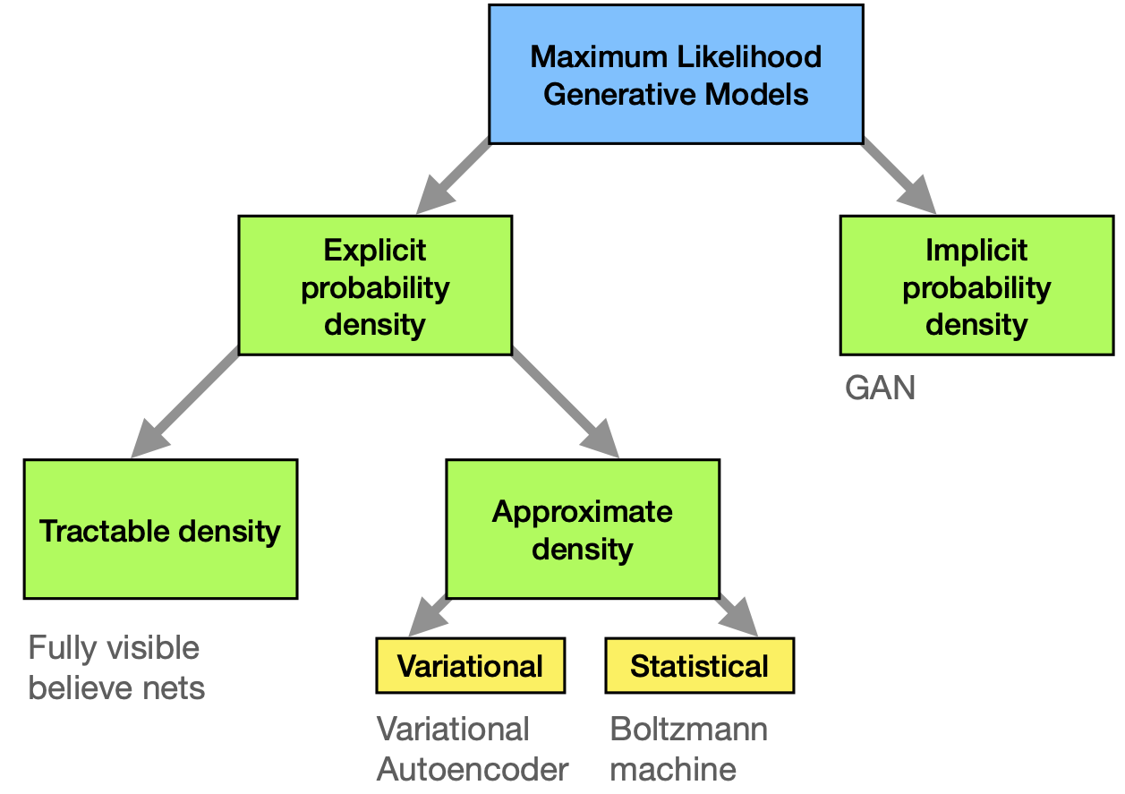
Fig. 28 Maximum likelihood approaches to generative modeling.
We restrict ourselves to methods that are based on the maximum likelihood principle. The role of the model is to provide an estimate \(p_{\text{model}}(\mathbf{x};\boldsymbol \theta)\) of a probability distribution parametrized by parameters \(\boldsymbol \theta\). The likelihood is the probability that the model assigns to the training data
where \(m\) is again the number of samples in the data \(\{\mathbf{x}_i\}\). The goal is to choose the parameters \(\boldsymbol \theta\) such as to maximize the likelihood. Thanks to the equality
we can just as well work with the sum of logarithms, which is easier to handle. As we explained previously (see section on t-SNE), the maximization is equivalent to the minimization of the cross-entropy between two probability distributions: the ‘true’ distribution \(p_{\mathrm{data}}(\mathbf{x})\) from which the data has been drawn and \(p_{\text{model}}(\mathbf{x};\boldsymbol \theta)\). While we do not have access to \(p_{\mathrm{data}}(\mathbf{x})\) in principle, we estimate it empirically as a distribution peaked at the \(m\) data points we have.
Methods can now be distinguished by the way \(p_{\mathrm{model}}\) is defined and evaluated (see Fig. 28). We differentiate between models that define \(p_{\mathrm{data}}(\mathbf{x})\) explicitly through some functional form. They have the general advantage that maximization of the likelihood is rather straight-forward, since we have direct access to this function. The downside is that the functional forms are generically limiting the ability of the model to fit the data distribution or become computationally intractable.
Among those explicit density models, we can further distinguish between those that represent a computationally tractable density and those that do not. An example for tractable explicit density models are fully visible belief networks (FVBNs) that decompose the probability distribution over an \(n\)-dimensional vector \(\mathbf{x}\) into a product of conditional probabilities
We can already see that, once we use the model to draw new samples, this is done one entry of the vector \(\mathbf{x}\) at a time (first \(x_1\) is drawn, then, knowing it, \(x_2\) is drawn etc.). This is computationally costly and not parallelizable but is useful for tasks that are anyway sequential (like generation of human speech, where the so-called WaveNet employs FVBNs).
Models that encode an explicit density, but require approximations to maximize the likelihood that can either be variational in nature or use stochastic methods. We have seen examples for either. Variational methods define a lower bound to the log likelihood which can be maximized
The algorithm produces a maximum value of the log-likelihood that is at least as high as the value for \(\mathcal{L}\) obtained (when summed over all data points). Variational autoencoders belong to this category. Their most obvious shortcoming is that \(\mathcal{L}(\mathbf{x};\boldsymbol \theta)\) may represent a very bad lower bound to the log-likelihood (and is in general not guaranteed to converge to it for infinite model size), so that the distribution represented by the model is very different from \(p_{\mathrm{data}}\). Stochastic methods, in contrast, often rely on a Markov chain process: The model is defined by a probability \(q(\mathbf{x}'|\mathbf{x})\) from which the current sample \(\mathbf{x}'\) is drawn, which depends on the previously drawn sample \(\mathbf{x}\) (but not any others). RBMs are an example for this. They have the advantage that there is some rigorously proven convergence to \(p_{\text{model}}\) with large enough size of the RBM, but the convergence may be slow. Like with FVBNs, the drawing process is sequential and thus not easily parallelizable.
All these classes of models allow for explicit representations of the probability density function approximations. In contrast, for GANs and related models, there is only an indirect access to said probability density: The model allows us to sample from it. Naturally, this makes optimization potentially harder, but circumvents many of the other previously mentioned problems. In particular
GANs can generate samples in parallel
there are few restrictions on the form of the generator function (as compared to Boltzmann machines, for instance, which have a restricted form to make Markov chain sampling work)
no Markov chains are needed
no variational bound is needed and some GAN model families are known to be asymptotically consistent (meaning that for a large enough model they are approximations to any probability distribution).
GANs have been immensely successful in several application scenarios. Their superiority against other methods is, however, often assessed subjectively. Most of performance comparison have been in the field of image generation, and largely on the ImageNet database. Some of the standard tasks evaluated in this context are:
generate an image from a sentence or phrase that describes its content (“a blue flower”)
generate realistic images from sketches
generate abstract maps from satellite photos
generate a high-resolution (“super-resolution”) image from a lower resolution one
predict a next frame in a video.
As far as more science-related applications are concerned, GANs have been used to
predict the impact of climate change on individual houses
generate new molecules that have been later synthesized.
In the light of these examples, it is of fundamental importance to understand that GANs enable (and excel at) problems with multi-modal outputs. That means the problems are such that a single input corresponds to many different ‘correct’ or ‘likely’ outputs. (In contrast to a mathematical function, which would always produce the same output.) This is important to keep in mind in particular in scientific applications, where we often search for the one answer. Only if that is not the case, GANs can actually play out their strengths.
Let us consider image super-resolution as an illustrative example: Conventional (deterministic) methods of increasing image resolution would necessarily lead to some blurring or artifacts, because the information that can be encoded in the finer pixel grid simply is not existent in the input data. A GAN, in contrast, will provide a possibility how a realistic image could have looked if it had been taken with higher resolution. This way they add information that may differ from the true scene of the image that was taken – a process that is obviously not yielding a unique answer since many versions of the information added may correspond to a realistic image.
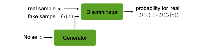
Fig. 29 Architecture of a GAN.
The working principle of GANs
The optimization of all neural network models we discussed so far was formulated as minimization of a cost function. For GANs, while such a formulation is a also possible, a much more illuminating perspective is viewing the GAN as a game between two players, the generator (\(G\)) and the discriminator (\(D\)), see Fig. 29. The role of \(G\) is to generate from some random input \(\mathbf{z}\) drawn from a simple distribution samples that could be mistaken from being drawn from \(p_{\mathrm{data}}\). The task of \(D\) is to classify its input as generated by \(G\) or coming from the data. Training should improve the performance of both \(D\) and \(G\) at their respective tasks simultaneously. After training is completed, \(G\) can be used to draw samples that closely resembles those drawn from \(p_{\mathrm{data}}\). In summary
where we have also indicated the two sets of parameters on which the two functions depend: \(\boldsymbol \theta_D\) and \(\boldsymbol \theta_G\), respectively. The game is then defined by two cost functions. The discriminator wants to minimize \(J_D(\boldsymbol \theta_D,\boldsymbol \theta_G)\) by only changing \(\boldsymbol \theta_D\), while the generator \(J_G(\boldsymbol \theta_D,\boldsymbol \theta_G)\) by only changing \(\boldsymbol \theta_G\). So, each players cost depends on both their and the other players parameters, the latter of which cannot be controlled by the player. The solution to this game optimization problem is a (local) minimum, i.e., a point in \((\boldsymbol \theta_D,\boldsymbol \theta_G)\)-space where \(J_D(\boldsymbol \theta_D,\boldsymbol \theta_G)\) has a local minimum with respect to \(\boldsymbol \theta_D\) and \(J_G(\boldsymbol \theta_D,\boldsymbol \theta_G)\) has a local minimum with respect to \(\boldsymbol \theta_G\). In game theory such a solution is called a Nash equilibrium. Let us now specify possible choices for the cost functions as well as for \(D\) and \(G\).
The most important requirement of \(G\) is that it is differentiable. It thus can (in contrast to VAEs) not have discrete variables on the output layer. A typical representation is a deep (possibly convolutional) neural network. A popular Deep Conventional architecture is called DCGAN. Then \(\boldsymbol \theta_G\) are the networks weights and biases. The input \(\mathbf{z}\) is drawn from some simple prior distribution, e.g., the uniform distribution or a normal distribution. (The specific choice of this distribution is secondary, as long as we use the same during training and when we use the generator by itself.) It is important that \(\mathbf{z}\) has at least as high a dimension as \(\mathbf{x}\) if the full multi-dimensional \(p_{\text{model}}\) is to be approximated. Otherwise the model will perform some sort of dimensional reduction. Several tweaks have also been used, such as feeding some components of \(\mathbf{z}\) into a hidden instead of the input layer and adding noise to hidden layers.
The training proceeds in steps. At each step, a minibatch of \(\mathbf{x}\) is drawn from the data set and a minibatch of \(\mathbf{z}\) is sampled from the prior distribution. Using this, gradient descent-type updates are performed: One update of \(\boldsymbol \theta_D\) using the gradient of \(J_D(\boldsymbol \theta_D,\boldsymbol \theta_G)\) and one of \(\boldsymbol \theta_G\) using the gradient of \(J_G(\boldsymbol \theta_D,\boldsymbol \theta_G)\).
The cost functions
For \(D\), the cost function of choice is the cross-entropy as with standard binary classifiers that have sigmoid output. Given that the labels are ‘1’ for data and ‘0’ for \(\mathbf{z}\) samples, it is simply
where the sums over \(i\) and \(j\) run over the respective minibatches, which contain \(N_1\) and \(N_2\) points.
For \(G\) more variations of the cost functions have been explored. Maybe the most intuitive one is
which corresponds to the so-called zero-sum or minmax game. Its solution is formally given by
This form of the cost is convenient for theoretical analysis, because there is only a single target function, which helps drawing parallels to conventional optimization. However, other cost functions have been proven superior in practice. The reason is that minimization can get trapped very far from an equilibrium: When the discriminator manages to learn rejecting generator samples with high confidence, the gradient of the generator will be very small, making its optimization very hard.
Instead, we can use the cross-entropy also for the generator cost function (but this time from the generator’s perspective)
Now the generator maximizes the probability of the discriminator being mistaken. This way, each player still has a strong gradient when the player is loosing the game. We observe that this version of \(J_G(\boldsymbol \theta_D,\boldsymbol \theta_G)\) has no direct dependence of the training data. Of course, such a dependence is implicit via \(D\), which has learned from the training data. This indirect dependence also acts like a regularizer, preventing overfitting: \(G\) has no possibility to directly ‘fit’ its output to training data.
Remarks
In closing this section, we comment on a few properties of GANs, which also mark frontiers for improvements. One global problem is that GANs are typically difficult to train: they require large training sets and are highly susceptible to hyper-parameter fluctuations. It is currently an active topic of research to compensate for this with the structural modification and novel loss function formulations.
Mode collapse
This may describe one of the most obvious problems of GANs: it refers to a situation where \(G\) does not explore the full space to which \(\mathbf{x}\) belongs, but rather maps several inputs \(\mathbf{z}\) to the same output. Mode collapse can be more or less severe. For instance a \(G\) trained on generating images may always resort to certain fragments or patterns of images. A formal reason for mode collapse is when the simultaneous gradient descent gravitates towards a solution
instead of the order in Eq. (47). (A priori it is not clear which of the two solutions is closer to the algorithm’s doing.) Note that the interchange of min and max in general corresponds to a different solution: It is now sufficient for \(G\) to always produce one (and the same) output that is classified as data by \(D\) with very high probability. Due to the mode collapse problem, GANs are not good at exploring ergodically the full space of possible outputs. They rather produce few very good possible outputs.
One strategy to fight mode collapse is called minibatch features. Instead of letting \(D\) rate one sample at a time, a minibatch of real and generated samples is considered at once. It then detects whether the generated samples are unusually close to each other.
Arithmetics with GANs
It has been demonstrated that GANs can do linear arithmetics with inputs to add or remove abstract features from the output. This has been demonstrated using a DCGAN trained on images of faces. The gender and the feature ‘wearing glasses’ can be added or subtracted and thus changed at will. Of course such a result is only empirical, there is no formal mathematical theory why it works.
Using GANs with labelled data
It has been shown that, if (partially) labeled data is available, using the labels when training \(D\) may improve the performance of \(G\). In this constellation, \(G\) has still the same task as before and does not interact with the labels. If data with \(n\) classes exist, then \(D\) will be constructed as a classifier for \((n+1)\) classes, where the extra class corresponds to ‘fake’ data that \(D\) attributes to coming from \(G\). If a data point has a label, then this label is used as a reference in the cost function. If a datapoint has no label, then the first \(n\) outputs of \(D\) are summed up.
One-sided label smoothing
This technique is useful not only for the \(D\) in GANs but also other binary classification problems with neural networks. Often we observe that classifiers give proper results, but show a too confident probability. This overshooting confidence can be counteracted by one-sided label smoothing. The idea is to simply replace the target value for the real examples with a value slightly less than 1, e.g., 0.9. This smoothes the distribution of the discriminator. Why do we only perform this off-set one-sided and not also give a small nonzero value \(\beta\) to the fake samples target values? If we were to do this, the optimal function for \(D\) is
Consider now a range of \(\mathbf{x}\) for which \(p_{\mathrm{data}}(\mathbf{x})\) is small but \(p_{\mathrm{model}}(\mathbf{x})\) is large (a “spurious mode”). \(D^\star(\mathbf{x})\) will have a peak near this spurious mode. This means \(D\) reinforces incorrect behavior of \(G\). This will encourage \(G\) to reproduce samples that it already makes (irrespective of whether they are anything like real data).
- 1
following “NIPS 2016 Tutorial: Generative Adversarial Netoworks” Ian Goodfellow, arXiv:1701.001160