
t-SNE as a Nonlinear Visualization Technique
We studied (kernel) PCA as an example for a method that reduces the dimensionality of a dataset and makes features apparent by which data points can be efficiently distinguished. Often, it is desirable to more clearly cluster similar data points and visualize this clustering in a low (two- or three-) dimensional space. We focus our attention on a relatively recent algorithm (from 2008) that has proven very performant. It goes by the name t-distributed stochastic neighborhood embedding (t-SNE).
The basic idea is to think of the data (images, for instance) as objects \(\mathbf{x}_i\) in a very high-dimensional space and characterize their relation by the Euclidean distance \(||\mathbf{x}_i-\mathbf{x}_j||\) between them. These pairwise distances are mapped to a probability distribution \(p_{ij}\). The same is done for the distances \(||\mathbf{y}_i-\mathbf{y}_j||\) of the images of the data points \(\mathbf{y}_i\) in the target low-dimensional space. Their probability distribution is denoted \(q_{ij}\). The mapping is optimized by changing the locations \(\mathbf{y}_i\) so as to minimize the distance between the two probability distributions. Let us substantiate these words with formulas.
The probability distribution in the space of data points is given as the symmetrized version (joint probability distribution)
of the conditional probabilities
where the choice of variances \(\sigma_i\) will be explained momentarily. Distances are thus turned into a Gaussian distribution. Note that \(p_{j|i}\neq p_{i|j}\) while \(p_{ji}= p_{ij}\).
The probability distribution in the target space is chosen to be a Student t-distribution
This choice has several advantages: (i) it is symmetric upon interchanging \(i\) and \(j\), (ii) it is numerically more efficiently evaluated because there are no exponentials, (iii) it has ‘fatter’ tails which helps to produce more meaningful maps in the lower dimensional space.
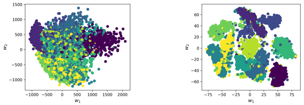
Fig. 6 PCA vs. t-SNE Application of both methods on 5000 samples from the MNIST handwritten digit dataset. We see that perfect clustering cannot be achieved with either method, but t-SNE delivers the much better result.
Let us now discuss the choice of \(\sigma_i\). Intuitively, in dense regions of the dataset, a smaller value of \(\sigma_i\) is usually more appropriate than in sparser regions, in order to resolve the distances better. Any particular value of \(\sigma_i\) induces a probability distribution \(P_i\) over all the other data points. This distribution has an entropy (here we use the Shannon entropy, in general it is a measure for the “uncertainty” represented by the distribution)
The value of \(H(P_i)\) increases as \(\sigma_i\) increases, i.e., the more uncertainty is added to the distances. The algorithm searches for the \(\sigma_i\) that result in a \(P_i\) with fixed perplexity
The target value of the perplexity is chosen a priory and is the main parameter that controls the outcome of the t-SNE algorithm. It can be interpreted as a smooth measure for the effective number of neighbors. Typical values for the perplexity are between 5 and 50.
Finally, we have to introduce a measure for the similarity between the two probability distributions \(p_{ij}\) and \(q_{ij}\). This defines a so-called loss function. Here, we choose the Kullback-Leibler divergence
which we will frequently encounter during this lecture. The symmetrized \(p_{ij}\) ensures that \(\sum_j p_{ij}>1/(2n)\), so that each data point makes a significant contribution to the cost function. The minimization of \(L(\{\mathbf{y}_i\})\) with respect to the positions \(\mathbf{y}_i\) can be achieved with a variety of methods. In the simplest case it can be gradient descent, which we will discuss in more detail in a later chapter. As the name suggests, it follows the direction of largest gradient of the cost function to find the minimum. To this end it is useful that these gradients can be calculated in a simple form
By now, t-SNE is implemented as standard in many packages. They involve some extra tweaks that force points \(\mathbf{y}_i\) to stay close together at the initial steps of the optimization and create a lot of empty space. This facilitates the moving of larger clusters in early stages of the optimization until a globally good arrangement is found. If the dataset is very high-dimensional it is advisable to perform an initial dimensionality reduction (to somewhere between 10 and 100 dimensions, for instance) with PCA before running t-SNE.
While t-SNE is a very powerful clustering technique, it has its limitations. (i) The target dimension should be 2 or 3, for much larger dimensions ansatz for \(q_{ij}\) is not suitable. (ii) If the dataset is intrinsically high-dimensional (so that also the PCA pre-processing fails), t-SNE may not be a suitable technique. (iii) Due to the stochastic nature of the optimization, results are not reproducible. The result may end up looking very different when the algorithm is initialized with some slightly different initial values for \(\mathbf{y}_i\).