
Restricted Boltzmann Machine
Restricted Boltzmann Machines (RBM) are a class of generative stochastic neural networks. More specifically, given some (binary) input data \(\mathbf{x}\in\{0,1\}^{n_v}\), an RBM can be trained to approximate the probability distribution of this input. Moreover, once the neural network is trained to approximate the distribution of the input, we can sample from the network, in other words we generate new instances from the learned probability distribution.
The RBM consists of two layers (see Fig. 22) of binary units. Each binary unit is a variable which can take the values \(0\) or \(1\). We call the first (input) layer visible and the second layer hidden. The visible layer with input variables \(\lbrace v_{1}, v_{2}, \dots v_{n_{\mathrm{v}}}\rbrace\), which we collect in the vector \(\mathbf{v}\), is connected to the hidden layer with variables \(\{ h_{1}, h_{2}, \dots h_{n_{\mathrm{h}}}\}\), which we collect in the vector \(\mathbf{h}\). The role of the hidden layer is to mediate correlations between the units of the visible layer. In contrast to the neural networks we have seen in the previous chapter, the hidden layer is not followed by an output layer. Instead, the RBM represents a probability distribution \(P_{\text{rbm}}(\mathbf{v})\), which depends on variational parameters represented by the weights and biases of a neural network. The RBM, as illustrated by the graph in Fig. 22, is a special case of a network structure known as a Boltzmann machine with the restriction that a unit in the visible layer is only connected to hidden units and vice versa, hence the name restricted Boltzmann machine.
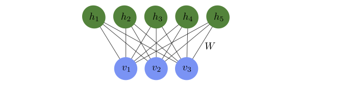
Fig. 22 Restricted Boltzmann machine. Each of the three visible units and five hidden units represents a variable that can take the values \(\pm1\) and the connections between them represent the entries \(W_{ij}\) of the weight matrix that enters the energy function (38).
The structure of the RBM is motivated from statistical physics: To each choice of the binary vectors \(\mathbf{v}\) and \(\mathbf{h}\), we assign a value we call the energy
where the vectors \(\mathbf{a}\), \(\mathbf{b}\), and the matrix \(W\) are the variational parameters of the model. Given the energy, the probability distribution over the configurations \((\mathbf{v}, \mathbf{h})\) is defined as
where
is a normalisation factor called the partition function. The sum in Eq. (40) runs over all binary vectors \(\mathbf{v}\) and \(\mathbf{h}\), i.e., vectors with entries \(0\) or \(1\). The probability that the model assigns to a visible vector \(\mathbf{v}\) is then the marginal over the joint probability distribution Eq. (39),
As a result of the restriction, the visible units, with the hidden units fixed, are mutually independent: given a choice of the hidden units \(\mathbf{h}\), we have an independent probability distribution for each visible unit given by
where \(\sigma(x) = 1/(1+e^{-x})\) is the sigmoid function. Similarly, with the visible units fixed, the individual hidden units are also mutually independent with the probability distribution
The visible (hidden) units can thus be interpreted as artificial neurons connected to the hidden (visible) units with sigmoid activation function and bias \(\mathbf{a}\) (\(\mathbf{b}\)). A direct consequence of this mutual independence is that sampling a vector \(\mathbf{v}\) or \(\mathbf{h}\) reduces to sampling every component individually. Notice that this simplification comes about due to the restriction that visible (hidden) units do not directly interact amongst themselves, i.e. there are no terms proportional to \(v_i v_j\) or \(h_i h_j\) in Eq. (38). In the following, we explain how one can train an RBM and discuss possible applications of RBMs.
Training an RBM
Consider a set of binary input data \(\mathbf{x}_k\), \(k=1,\ldots,M\), drawn from a probability distribution \(P_{\textrm{data}}(\mathbf{x})\). The aim of the training is to tune the parameters \(\lbrace \mathbf{a}, \mathbf{b}, W \rbrace\) in an RBM such that after training \(P_{\textrm{rbm}}(\mathbf{x}) \approx P_{\textrm{data}}(\mathbf{x})\). The standard approach to solve this problem is the maximum likelihood principle, in other words we want to find the parameters \(\lbrace \mathbf{a}, \mathbf{b}, W \rbrace\) which maximize the probability that our model produces the data \(\mathbf{x}_k\).
Maximizing the likelihood \(\mathcal{L}(\mathbf{a},\mathbf{b},W) = \prod P_{\textrm{rbm}}(\mathbf{x}_{k})\) is equivalent to training the RBM using a loss function we have encountered before, the negative log-likelihood
For the gradient descent, we need derivatives of the loss function of the form
This derivative consists of two terms,
and similarly simple forms are found for the derivatives with respect to the components of \(\mathbf{a}\) and \(\mathbf{b}\). We can then iteratively update the parameters just as we have done in Chapter Computational neurons,
with a sufficiently small learning rate \(\eta\). As we have seen in the previous chapter in the context of backpropagation, we can reduce the computational cost by replacing the summation over the whole data set in Eq. (43) with a summation over a small randomly chosen batch of samples. This reduction in the computational cost comes at the expense of noise, but at the same time it can help to improve generalization.
However, there is one more problem: The second summation in Eq. (44), which contains \(2^{n_v}\) terms, cannot be efficiently evaluated exactly. Instead, we have to approximate the sum by sampling the visible layer \(\mathbf{v}\) from the marginal probability distribution \(P_{\textrm{rbm}}(\mathbf{v})\). This sampling can be done using Gibbs sampling as follows:
Gibbs-Sampling
Input: Any visible vector \(\mathbf{v}(0)\)
Output: Visible vector \(\mathbf{v}(r)\)
for: \(n=1\)\dots \(r\)
\(\quad\) sample \(\mathbf{h}(n)\) from \(P_{\rm rbm}(\mathbf{h}|\mathbf{v}=\mathbf{v}(n-1))\)
\(\quad\) sample \(\mathbf{v}(n)\) from \(P_{\rm rbm}(\mathbf{v}|\mathbf{h}=\mathbf{h}(n))\)
end
With sufficiently many steps \(r\), the vector \(\mathbf{v}(r)\) is an unbiased sample drawn from \(P_{\textrm{rbm}}(\mathbf{v})\). By repeating the procedure, we can obtain multiple samples to estimate the summation. Note that this is still rather computationally expensive, requiring multiple evaluations on the model.
The key innovation which allows the training of an RBM to be computationally feasible was proposed by Geoffrey Hinton (2002). Instead of obtaining multiple samples, we simply perform the Gibbs sampling with \(r\) steps and estimate the summation with a single sample, in other words we replace the second summation in Eq. (44) with
where \(\mathbf{v}' = \mathbf{v}(r)\) is simply the sample obtained from \(r\)-step Gibbs sampling. With this modification, the gradient, Eq. (44), can be approximated as
This method is known as contrastive divergence. Although the quantity computed is only a biased estimator of the gradient, this approach is found to work well in practice. The complete algorithm for training a RBM with \(r\)-step contrastive divergence can be summarised as follows:
Contrastive divergence
Input: Dataset \(\mathcal{D} = \lbrace \ \mathbf{x}_{1}, \ \mathbf{x}_{2}, \dots \ \mathbf{x}_{M} \rbrace\) drawn from a distribution \(P(x)\)}
initialize the RBM weights \(\lbrace \mathbf{a},\mathbf{b},W \rbrace\)
Initialize \(\Delta W_{ij} = \Delta a_{i} = \Delta b_{j} =0\)
while: not converged do
\(\quad\) select a random batch \(S\) of samples from the dataset \(\mathcal{D}\)
\(\quad\) forall \(\mathbf{x} \in S\)
\(\quad\quad\) Obtain \(\ \mathbf{v}'\) by \(r\)-step Gibbs sampling starting from \(\ \mathbf{x}\)
\(\quad\quad\) \(\Delta W_{ij} \leftarrow \Delta W_{ij} - x_{i}P_{\textrm{rbm}}(h_{j}=1|\ \mathbf{x}) + v'_{i} P_{\textrm{rbm}}(h_{j}=1|\ \mathbf{h}')\)
\(\quad\) end
\(\quad\) \(W_{ij} \leftarrow W_{ij} - \eta\Delta W_{ij}\)
\(\quad\) (and similarly for \(\mathbf{a}\) and \(\mathbf{b}\))
end
Having trained the RBM to represent the underlying data distribution \(P(\mathbf{x})\), there are a few ways one can use the trained model:
Pretraining: We can use \(W\) and \(\mathbf{b}\) as the initial weights and biases for a deep network (c.f. Chapter 4), which is then fine-tuned with gradient descent and backpropagation.
Generative Modelling: As a generative model, a trained RBM can be used to generate new samples via Gibbs sampling. Some potential uses of the generative aspect of the RBM include recommender systems and image reconstruction. In the following subsection, we provide an example, where an RBM is used to reconstruct a noisy signal.
Example: signal or image reconstruction/denoising
A major drawback of the simple RBMs for their application is the fact that they only take binary data as input. As an example, we thus look at simple periodic waveforms with 60 sample points. In particular, we use sawtooth, sine, and square waveforms. In order to have quasi-continuous data, we use eight bits for each point, such that our signal can take values from 0 to 255. Finally, we generate samples to train with a small variation in the maximum value, the periodicity, as well as the center point of each waveform.
After training the RBM using the contrastive divergence algorithm, we now have a model which represents the data distribution of the binarized waveforms. Consider now a signal which has been corrupted, meaning some parts of the waveform have not been received, in other words they are set to 0. By feeding this corrupted data into the RBM and performing a few iterations of Gibbs sampling, we can obtain a reconstruction of the signal, where the missing part has been repaired, as can been seen at the bottom of Fig. 23.
Note that the same procedure can be used to reconstruct or denoise images. Due to the limitation to binary data, however, the picture has to either be binarized, or the input size to the RBM becomes fairly large for high-resolution pictures. It is thus not surprising that while RBMs have been popular in the mid-2000s, they have largely been superseded by more modern and architectures such as generative adversarial networks which we shall explore later in the chapter. However, they still serve a pedagogical purpose and could also provide inspiration for future innovations, in particular in science. A recent example is the idea of using an RBM to represent a quantum mechanical state.
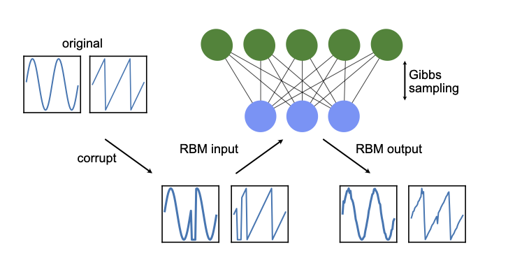
Fig. 23 Signal reconstruction. Using an RBM to repair a corrupted signal, here a sine and a sawtooth waveform.