
Kernel PCA
PCA performs a linear transformation on the data. However, there are cases where such a transformation is unable to produce any meaningful result. Consider for instance the fictitious dataset with \(2\) classes and \(2\) data features as shown on the left of Fig. 5. We see by naked eye that it should be possible to separate this data well, for instance by the distance of the datapoint from the origin, but it is also clear that a linear function cannot be used to compute it. In this case, it can be helpful to consider a non-linear extension of PCA, known as kernel PCA.
The basic idea of this method is to apply to the data \(\mathbf{x} \in \mathbb{R}^{n}\) a chosen non-linear vector-valued transformation function \(\mathbf{\Phi}(\mathbf{x})\) with
which is a map from the original \(n\)-dimensional space (corresponding to the \(n\) original data features) to a \(N\)-dimensional feature space. Kernel PCA then simply involves performing the standard PCA on the transformed data \(\mathbf{\Phi}(\mathbf{x})\). Here, we will assume that the transformed data is centered, i.e.,
to have simpler formulas.
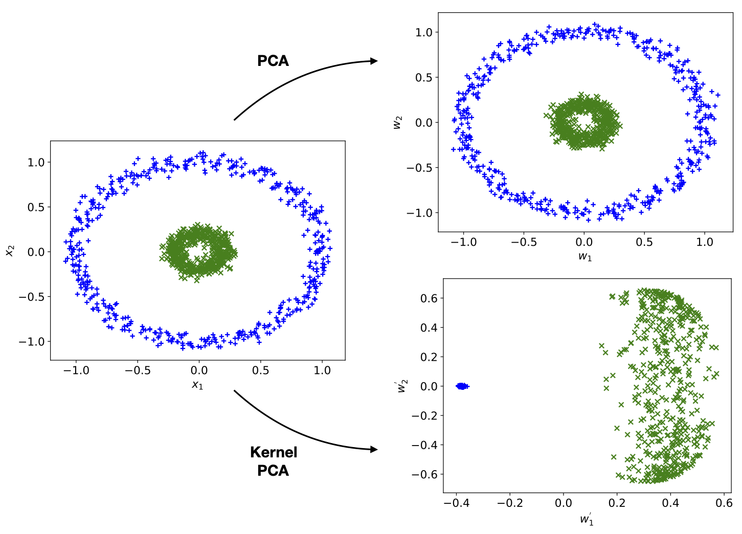
Fig. 5 Kernel PCA versus PCA.
In practice, when \(N\) is large, it is not efficient or even possible to explicitly perform the transformation \(\mathbf{\Phi}\). Instead we can make use of a method known as the kernel trick. Recall that in standard PCA, the primary aim is to find the eigenvectors and eigenvalues of the covariance matrix \(C\) . In the case of kernel PCA, this matrix becomes
with the eigenvalue equation
By writing the eigenvectors \(\mathbf{v}_{j}\) as a linear combination of the transformed data features
we see that finding the eigenvectors is equivalent to finding the coefficients \(a_{ji}\). On substituting this form back into Eq. (4), we find
By multiplying both sides of the equation by \(\mathbf{\Phi}(\mathbf{x}_{k})^{T}\) we arrive at
where \(K(\mathbf{x},\mathbf{y}) = \mathbf{\Phi}(\mathbf{x})^{T} \mathbf{\Phi}(\mathbf{y})\) is known as the kernel. Thus we see that if we directly specify the kernels we can avoid explicit performing the transformation \(\mathbf{\Phi}\). In matrix form, we find the eigenvalue equation \(K^{2}\mathbf{a}_{j} = \lambda_{j} K \mathbf{a}_{j}\), which simplifies to
Note that this simplification requires \(\lambda_j \neq 0\), which will be the case for relevant principle components. (If \(\lambda_{j} = 0\), then the corresponding eigenvectors would be irrelevant components to be discarded.) After solving the above equation and obtaining the coefficients \(a_{jl}\), the kernel PCA transformation is then simply given by the overlap with the eigenvectors \(\mathbf{v}_{j}\), i.e.,
where once again the explicit \(\mathbf{\Phi}\) transformation is avoided.
A common choice for the kernel is known as the radial basis function kernel (RBF) defined by
where \(\gamma\) is a tunable parameter. Using the RBF kernel, we compare the result of kernel PCA with that of standard PCA, as shown on the right of Fig. 5. It is clear that kernel PCA leads to a meaningful separation of the data while standard PCA completely fails.