
Dreaming and the Problem of Extrapolation
Exploring the weights and intermediate activations of a neural network in order to understand what the network has learnt, very quickly becomes unfeasible or uninformative for large network architectures. In this case, we can try a different approach, where we focus on the inputs to the neural network, rather than the intermediate activations.
More precisely, let us consider a neural network classifier \(\mathbf{f}\), depending on the weights \(W\), which maps an input \(\mathbf{x}\) to a probability distribution over \(n\) classes \(\mathbf{f}(\mathbf{x}|W) \in \mathbb{R}^{n}\), i.e.,
We want to minimise the distance between the output of the network \(\mathbf{f(\mathbf{x})}\) and a chosen target output \(\mathbf{y}_{\textrm{target}}\), which can be done by minimizing the loss function
However, unlike in supervised learning where the loss minimization was done with respect to the weights \(W\) of the network, here we are interested in minimizing with respect to the input \(\mathbf{x}\) while keeping the weights \(W\) fixed. This can be achieved using gradient descent, i.e.
where \(\eta\) is the learning rate. With a sufficient number of iterations, our initial input \(\mathbf{x}^{0}\) will be transformed into the final input \(\mathbf{x}^{*}\) such that
By choosing the target output to correspond to a particular class, e.g., \(\mathbf{y}_{\textrm{target}} = (1, 0, 0, \dots)\), we are then essentially finding examples of inputs which the network would classify as belonging to the chosen class. This procedure is called dreaming.
Let us apply this technique to a binary classification example. We consider a dataset 2 consisting of images of healthy and unhealthy plant leaves. Some samples from the dataset are shown in the top row of Fig. 30. After training a deep convolutional network to classify the leaves (reaching a test accuracy of around \(95\%\)), we start with a random image as our initial input \(\mathbf{x}^{0}\) and perform gradient descent on the input, as described above, to arrive at the final image \(\mathbf{x}^{*}\) which our network confidently classifies.
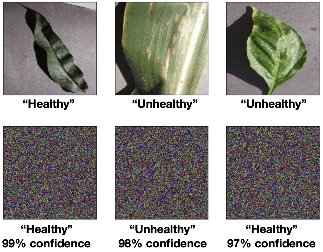
Fig. 30 Plant leaves. Top: Some samples from the plants dataset. Bottom: Samples generated by using the “dreaming” procedure starting from random noise.
In bottom row of Fig. 30, we show three examples produced using the ‘dreaming’ technique. On first sight, it might be astonishing that the final image actually does not even remotely resemble a leaf. How could it be that the network has such a high accuracy of around \(95\%\), yet we have here a confidently classified image which is essentially just noise. Although this seem surprising, a closer inspection reveals the problem: The noisy image \(\mathbf{x}^{*}\) looks nothing like the samples in the dataset with which we trained our network. By feeding this image into our network, we are asking it to make an extrapolation, which as can be seen leads to an uncontrolled behavior. This is a key issue which plagues most data driven machine learning approaches. With few exceptions, it is very difficult to train a model capable of performing reliable extrapolations. Since scientific research is often in the business of making extrapolations, this is an extremely important point of caution to keep in mind.
While it might seem obvious that any model should only be predictive for data that ‘resembles’ those in the training set, the precise meaning of ‘resembles’ is actually more subtle than one imagines. For example, if one trains a ML model using a dataset of images captured using a Canon camera but subsequently decide to use the model to make predictions on images taken with a Nikon camera, we could actually be in for a surprise. Even though the images may ‘resemble’ each other to our naked eye, the different cameras can have a different noise profile which might not be perceptible to the human eye. We shall see in the next section that even such minute image distortions can already be sufficient to completely confuse our model.
- 2
Source: https://data.mendeley.com/datasets/tywbtsjrjv/1