
Linear Regression
Linear regression, as the name suggests, simply means to fit a linear model to a dataset. Consider a dataset consisting of input-output pairs \(\lbrace(\mathbf{x}_{1}, y_{1}), \dots, (\mathbf{x}_{m}, y_{m})\rbrace\), where the inputs are \(n\)-component vectors \(\boldsymbol{x}^{T} = (x_1, x_2, \dots , x_n)\) and the output \(y\) is a real-valued number. The linear model then takes the form
or in matrix notation
where \(\mathbf{\tilde{x}}^{T} = (1, x_1, x_2, \dots , x_n)\) and \(\boldsymbol \beta = (\beta_0, \dots, \beta_n)^{T}\) are \((n+1)\) dimensional row vectors.
The aim then is to find parameters \(\hat{\boldsymbol \beta}\) such that \(f(\mathbf{x}|\hat{\boldsymbol \beta})\) is a good estimator for the output value \(y\). In order to quantify what it means to be a “good” estimator, one need to specify a real-valued loss function \(L(\boldsymbol \beta)\), sometimes also called a cost function. The good set of parameters \(\hat{\boldsymbol \beta}\) is then the minimizer of this loss function
There are many, inequivalent, choices for this loss function. For our purpose, we choose the loss function to be residual sum of squares (RSS) defined as
where the sum runs over the \(m\) samples of the dataset. This loss function is sometimes also called the L2-loss and can be seen as a measure of the distance between the output values from the dataset \(y_i\) and the corresponding predictions \(f(\mathbf{x}_i|\boldsymbol \beta)\).
It is convenient to define the \(m\) by \((n+1)\) data matrix \(\widetilde{X}\), each row of which corresponds to an input sample \(\mathbf{\tilde{x}}^{T}_{i}\), as well as the output vector \(\mathbf{Y}^{T} = (y_{1}, \dots, y_{m})\). With this notation, Eq. (10) can be expressed succinctly as a matrix equation
The minimum of \(\textrm{RSS}(\boldsymbol \beta)\) can be easily solved by considering the partial derivatives with respect to \(\boldsymbol \beta\), i.e.,
At the minimum, \(\frac{\partial \textrm{RSS}}{\partial \boldsymbol \beta} = 0\) and \(\frac{\partial^{2} \textrm{RSS}}{\partial \boldsymbol \beta\partial \boldsymbol \beta^{T}}\) is positive-definite. Assuming \(\widetilde{X}^{T}\widetilde{X}\) is full-rank and hence invertible, we can obtain the solution \(\hat{\boldsymbol \beta}\) as
If \(\widetilde{X}^{T}\widetilde{X}\) is not full-rank, which can happen if certain data features are perfectly correlated (e.g., \(x_1 = 2x_3\)), the solution to \(\widetilde{X}^{T}\widetilde{X}\boldsymbol \beta = \widetilde{X}^{T}\mathbf{Y}\) can still be found, but it would not be unique. Note that the RSS is not the only possible choice for the loss function and a different choice would lead to a different solution.
What we have done so far is uni-variate linear regression, that is linear regression where the output \(y\) is a single real-valued number. The generalisation to the multi-variate case, where the output is a \(p\)-component vector \(\mathbf{y}^{T} = (y_1, \dots y_p)\), is straightforward. The model takes the form
where the parameters \(\beta_{jk}\) now have an additional index \(k = 1, \dots, p\). Considering the parameters \(\beta\) as a \((n+1)\) by \(p\) matrix, we can show that the solution takes the same form as before [Eq. (11)] with \(Y\) as a \(m\) by \(p\) output matrix.
Statistical analysis
Let us stop here and evaluate the quality of the method we have just introduced. At the same time, we will take the opportunity to introduce some statistics notions, which will be useful throughout the book.
Up to now, we have made no assumptions about the dataset we are given, we simply stated that it consisted of input-output pairs, \(\{(\mathbf{x}_{1}, y_{1}), \dots,\) \((\mathbf{x}_{m}, y_{m})\}\). In order to assess the accuracy of our model in a mathematically clean way, we have to make an additional assumption. The output data \(y_1\ldots, y_m\) may arise from some measurement or observation. Then, each of these values will generically be subject to errors \(\epsilon_1,\cdots, \epsilon_m\) by which the values deviate from the “true” output without errors,
We assume that this error \(\epsilon\) is a Gaussian random variable with mean \(\mu = 0\) and variance \(\sigma^2\), which we denote by \(\epsilon \sim \mathcal{N}(0, \sigma^2)\). Assuming that a linear model in Eq. (8) is a suitable model for our dataset, we are interested in the following question: How does our solution \(\hat{\boldsymbol \beta}\) as given in Eq. (11) compare with the true solution \(\boldsymbol \beta^{\textrm{true}}\) which obeys
In order to make statistical statements about this question, we have to imagine that we can fix the inputs \(\mathbf{x}_{i}\) of our dataset and repeatedly draw samples for our outputs \(y_i\). Each time we will obtain a different value for \(y_i\) following Eq. (14), in other words the \(\epsilon_i\) are uncorrelated random numbers. This allows us to formalise the notion of an expectation value \(E(\cdots)\) as the average over an infinite number of draws. For each draw, we obtain a new dataset, which differs from the other ones by the values of the outputs \(y_i\). With each of these datasets, we obtain a different solution \(\hat{\boldsymbol \beta}\) as given by Eq. (11). The expectation value \(E(\hat{\boldsymbol \beta})\) is then simply the average value we obtained across an infinite number of datasets. The deviation of this average value from the “true” value given perfect data is called the bias of the model,
For the linear regression we study here, the bias is exactly zero, because
where the second line follows because \(E(\mathbf{\epsilon}) = \mathbf{0}\) and \((\widetilde{X}^{T}\widetilde{X})^{-1} \widetilde{X}^{T} \mathbf{Y}^{\textrm{true}} = \boldsymbol \beta^{\textrm{true}}\). Equation (16) implies linear regression is unbiased. Note that other machine learning algorithms will in general be biased.
What about the standard error or uncertainty of our solution? This information is contained in the covariance matrix
The covariance matrix can be computed for the case of linear regression using the solution in Eq. (11), the expectation value in Eq. (16) and the assumption in Eq. (14) that \(Y = Y^{\textrm{true}} + \mathbf{\epsilon}\) yielding
This expression can be simplified by using the fact that our input matrices \(\widetilde{X}\) are independent of the draw such that
Here, the second line follows from the fact that different samples are uncorrelated, which implies that \(E(\mathbf{\epsilon} \mathbf{\epsilon}^{T}) = \sigma^2 I\) with \(I\) the identity matrix. The diagonal elements of \(\sigma^2 (\widetilde{X}^{T}\widetilde{X})^{-1}\) then correspond to the variance
of the individual parameters \(\beta_i\). The standard error or uncertainty is then \(\sqrt{\textrm{Var}(\hat{\beta}_{i})}\).
There is one more missing element: we have not explained how to obtain the variances \(\sigma^2\) of the outputs \(y\). In an actual machine learning task, we would not know anything about the true relation, as given in Eq. (14), governing our dataset. The only information we have access to is a single dataset. Therefore, we have to estimate the variance using the samples in our dataset, which is given by
where \(y_i\) are the output values from our dataset and \(f(\mathbf{x}_i|\hat{\boldsymbol \beta})\) is the corresponding prediction. Note that we normalized the above expression by \((m - n - 1)\) instead of \(m\) to ensure that \(E(\hat{\sigma}^2) = \sigma^2\), meaning that \(\hat{\sigma}^2\) is an unbiased estimator of \(\sigma^2\).
Our ultimate goal is not simply to fit a model to the dataset. We want our model to generalize to inputs not within the dataset. To assess how well this is achieved, let us consider the prediction \(\tilde{\mathbf{a}}^{T} \hat{\boldsymbol \beta}\) on a new random input-output pair \((\mathbf{a},y_{0})\). The output is again subject to an error \(y_{0} = \tilde{\mathbf{a}}^{T}\boldsymbol \beta^{\textrm{true}} + \epsilon\). In order to compute the expected error of the prediction, we compute the expectation value of the loss function over these previously unseen data. This is also known as the test or generalization error . For the square-distance loss function, this is the mean square error (MSE)
There are three terms in the expression. The first term is the irreducible or intrinsic uncertainty of the dataset. The second term represents the bias and the third term is the variance of the model. For RSS linear regression, the estimate is unbiased so that
Based on the assumption that the dataset indeed derives from a linear model as given by Eq. (14) with a Gaussian error, it can be shown that the RSS solution, Eq. (11), gives the minimum error among all unbiased linear estimators, Eq. (8). This is known as the Gauss-Markov theorem.
This completes our error analysis of the method.
Regularization and the bias-variance tradeoff
Although the RSS solution has the minimum error among unbiased linear estimators, the expression for the generalisation error, Eq. (17), suggests that we can actually still reduce the error by sacrificing some bias in our estimate.
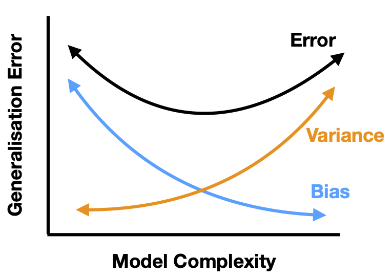
Fig. 7 Schematic depiction of the bias-variance tradeoff.
A possible way to reduce generalisation error is actually to drop some data features. From the \(n\) data features \(\lbrace x_{1}, \dots x_{n} \rbrace\), we can pick a reduced set \(\mathcal{M}\). For example, we can choose \(\mathcal{M} = \lbrace x_{1}, x_{3}, x_{7} \rbrace\), and define our new linear model as
This is equivalent to fixing some parameters to zero, i.e., \(\beta_k = 0\) if \(x_{k} \notin \mathcal{M}\). Minimizing the RSS with this constraint results in a biased estimator but the reduction in model variance can sometimes help to reduce the overall generalisation error. For a small number of features \(n \sim 20\), one can search exhaustively for the best subset of features that minimises the error, but beyond that the search becomes computationally unfeasible.
A common alternative is called ridge regression. In this method, we consider the same linear model given in Eq. (8) but with a modified loss function
where \(\lambda > 0\) is a positive parameter. This is almost the same as the RSS apart from the term proportional to \(\lambda\) [c.f. Eq. (10){]. The effect of this new term is to penalize large parameters \(\beta_j\) and bias the model towards smaller absolute values. The parameter \(\lambda\) is an example of a hyper-parameter, which is kept fixed during the training. On fixing \(\lambda\) and minimising the loss function, we obtain the solution
from which we can see that as \(\lambda \rightarrow \infty\), \(\hat{\boldsymbol \beta}_{\textrm{ridge}} \rightarrow \mathbf{0}\). By computing the bias and variance,
it is also obvious that increasing \(\lambda\) increases the bias, while reducing the variance. This is the tradeoff between bias and variance. By appropriately choosing \(\lambda\) it is possible that generalisation error can be reduced. We will introduce in the next section a common strategy how to find the optimal value for \(\lambda\).
The techniques presented here to reduce the generalization error, namely dropping of features and biasing the model to small parameters, are part of a large class of methods known as regularization. Comparing the two methods, we can see a similarity. Both methods actually reduce the complexity of our model. In the former, some parameters are set to zero, while in the latter, there is a constraint which effectively reduces the magnitude of all parameters. A less complex model has a smaller variance but larger bias. By balancing these competing effects, generalisation can be improved, as illustrated schematically in Fig. 7.
In the next chapter, we will see that these techniques are useful beyond applications to linear methods. We illustrate the different concepts in the following example.
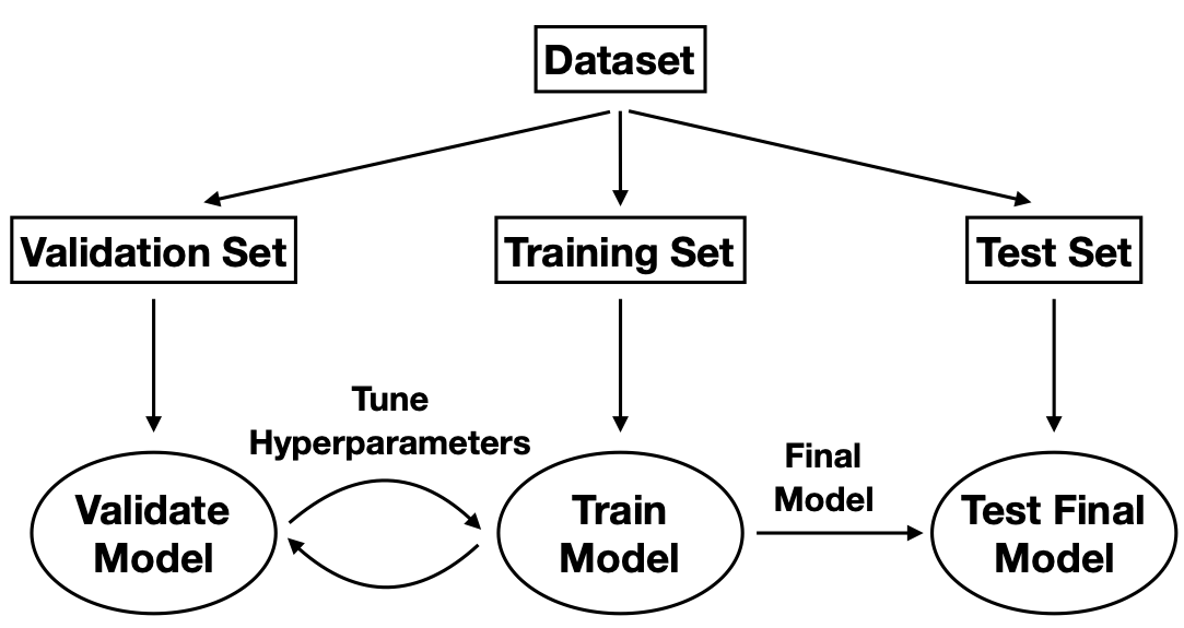
Fig. 8 Machine Learning Workflow.
Example
We illustrate the concepts of linear regression using a medical dataset. In the process, we will also familiarize ourselves with the standard machine learning workflow [see Fig. 8]. For this example, we are given \(10\) data features, namely age, sex, body mass index, average blood pressure, and six blood serum measurements from \(442\) diabetes patients, and our task is train a model \(f(\mathbf{x}|\boldsymbol \beta)\) [Eq. (8)] to predict a quantitative measure of the disease progression after one year.
Recall that the final aim of a machine-learning task is not to obtain the smallest possible value for the loss function such as the RSS, but to minimise the generalisation error on unseen data [c.f. Eq. (17)]. The standard approach relies on a division of the dataset into three subsets: training set, validation set and test set. The standard workflow is summarised in the Box below.
ML Workflow
Divide the dataset into training set \(\mathcal{T}\), validation set \(\mathcal{V}\) and test set \(\mathcal{S}\). A common ratio for the split is \(70 : 15 : 15\).
Pick the hyperparameters, e.g., \(\lambda\) in Eq. (19).
Train the model with only the training set, in other words minimize the loss function on the training set. [This corresponds to Eq. (11) or (20) for the linear regression, where \(\widetilde{X}\) only contains the training set.]
Evaluate the MSE (or any other chosen metric) on the validation set, [c.f. Eq. (17)]
\[\textrm{MSE}_{\textrm{validation}}(\hat{\boldsymbol \beta}) = \frac{1}{|\mathcal{V}|}\sum_{j\in\mathcal{V}} (y_j - f(\mathbf{x}_j|\hat{\boldsymbol \beta}))^2.\]This is known as the validation error.
Pick a different value for the hyperparameters and repeat steps \(3\) and \(4\), until validation error is minimized.
Evaluate the final model on the test set
\[\textrm{MSE}_{\textrm{test}}(\hat{\boldsymbol \beta}) = \frac{1}{|\mathcal{S}|}\sum_{j\in\mathcal{S}} (y_j - f(\mathbf{x}_j|\hat{\boldsymbol \beta}))^2.\]
It is important to note that the test set \(\mathcal{S}\) was not involved in optimizing either parameters \(\boldsymbol \beta\) or the hyperparameters such as \(\lambda\).
Applying this procedure to the diabetes dataset 2, we obtain the results in Fig. 9. We compare RSS linear regression with the ridge regression, and indeed we see that by appropriately choosing the regularisation hyperparameter \(\lambda\), the generalisation error can be minimized.
As side remark regarding the ridge regression, we can see on the left of Fig. 10, that as \(\lambda\) increases, the magnitude of the parameters, Eq. (20), \(\hat{\boldsymbol \beta}_{\textrm{ridge}}\) decreases. Consider on the other hand, a different form of regularisation, which goes by the name lasso regression, where the loss function is given by
Despite the similarities, lasso regression has a very different behaviour as depicted on the right of Fig. 10. Notice that as \(\alpha\) increases some parameters actually vanish and can be ignored completely. This actually corresponds to dropping certain data features completely and can be useful if we are interested in selecting the most important features in a dataset.
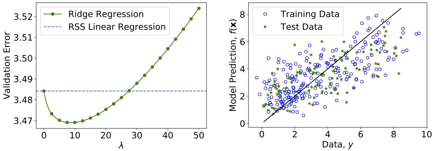
Fig. 9 Ridge Regression on Diabetes patients dataset. Left: Validation error versus \(\lambda\). Right: Test data versus the prediction from the trained model. If the prediction were free of any error, all the points would fall on the blue line.
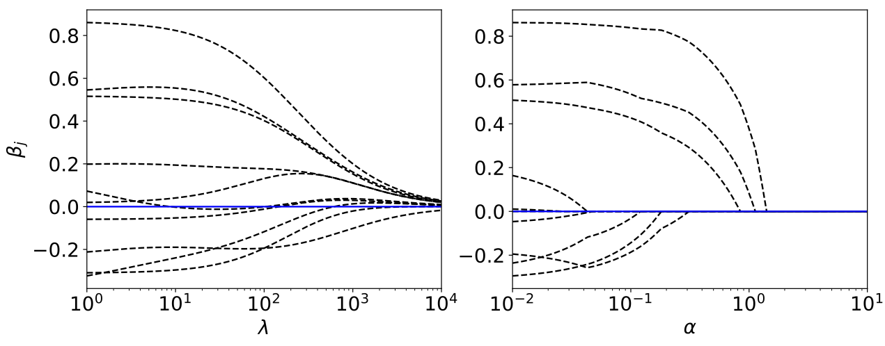
Fig. 10 Evolution of the model parameters. Increasing the hyperparameter \(\lambda\) or \(\alpha\) leads to a reduction of the absolute value of the model parameters, here shown for the ridge (left) and Lasso (right) regression for the Diabetes dataset.