
Recurrent neural networks
We have seen in the previous section how the convolutional neural network allows to retain local information through the use of filters. While this context-sensitivity of the CNN is applicable in many situations, where geometric information is important, there are situations we have more than neighborhood relations, namely sequential order. An element is before or after an other, not simply next to it. A common situation, where the order of the input is important, is with time-series data. Examples are measurements of a distant star collected over years or the events recorded in a detector after a collision in a particle collider. The classification task in these examples could be the determination whether the star has an exoplanet, or whether a Higgs boson was observed, respectively. Another example without any temporal structure in the data is the prediction of a protein’s functions from its primary amino-acid sequence.
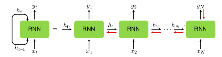
Fig. 20 Recurrent neural network architecture: The input \(x_t\) is fed into the recurrent cell together with the (hidden) memory \(h_{t-1}\) of the previous step to produce the new memory \(h_t\) and the output \(y_t\). One can understand the recurrent structure via the “unwrapped” depiction of the structure on the right hand side of the figure. The red arrows indicate how gradients are propagated back in time for updating the network parameters.
A property that the above examples have in common is that the length of the input data is not necessarily always fixed for all samples. This emphasizes again another weakness of both the dense network and the CNN: The networks only work with fixed-size input and there is no good procedure to decrease or increase the input size. While we can in principle always cut our input to a desired size, of course, this finite window is not guaranteed to contain the relevant information.
In this final section on supervised learning, we introduce one more neural network architecture that solves both problems discussed above: recurrent neural networks (RNNs). The key idea behind a recurrent neural network is that input is passed to the network one element after another—unlike for other neural networks, where an input ’vector’ is given the network all at once—and to recognize context, the network keeps an internal state, or memory, that is fed back to the network together with the next input. Recurrent neural networks were developed in the context of natural language processing (NLP), the field of processing, translating and transforming spoken or written language input, where clearly, both context and order are crucial pieces of information. However, over the last couple of years, RNNs have found applications in many fields in the sciences.
The special structure of a RNN is depicted in Fig. 20. At step \(t\), the input \({\boldsymbol{x}}_t\) and the (hidden) internal state of the last step \({\boldsymbol{h}}_{t-1}\) are fed to the network to calculate \({\boldsymbol{h}}_t\). The new hidden memory of the RNN is finally connected to the output layer \({\boldsymbol{y}}_t\). As shown in Fig. 20, this is equivalent to having many copies of the input-output architecture, where the hidden layers of the copies are connected to each other. The RNN cell itself can have a very simple structure with a single activation function. Concretely, in each step of a simple RNN we update the hidden state as
where we used for the nonlinearity the hyperbolic tangent, a common choice, which is applied element-wise. Further, if the input data \({\boldsymbol{x}}_t\) has dimension \(n\) and the hidden state \({\boldsymbol{h}}_t\) dimension \(m\), the weight matrices \(W_{hh}\) and \(W_{ih}\) have dimensions \(m\times m\) and \(m\times n\), respectively. Finally, the output at step \(t\) can be calculated using the hidden state \({\boldsymbol{h}}_t\),
A schematic of this implementation is depicted in Fig. 21(a). Note that in this simplest implementation, the output is only a linear operation on the hidden state. A straight forward extension—necessary in the case of a classification problem—is to add a non-linear element to the output as well, i.e.,
with \({\boldsymbol{g}}({\boldsymbol{q}})\) some activation function, such as a softmax. Note that while in principle an output can be calculated at every step, this is only done after the last input element in a classification task. An interesting property of RNNs is that the weight matrices and biases, the parameters we learn during training, are the same for each input element. This property is called parameter sharing and is in stark contrast to dense networks. In the latter architecture, each input element is connected through its own weight matrix. While it might seem that this property could be detrimental in terms of representability of the network, it can greatly help extracting sequential information: Similar to a filter in a CNN, the network does not need to learn the exact location of some specific sequence that carries the important information, it only learns to recognize this sequence somewhere in the data. Note that the way each input element is processed differently is instead implemented through the hidden memory.
Parameter sharing is, however, also the root of a major problem when training a simple RNN. To see this, remember that during training, we update the network parameters using gradient descent. As in the previous sections, we can use backpropagation to achieve this optimization. Even though the unwrapped representation of the RNN in Fig. 20 suggests a single hidden layer, the gradients for the backpropagation have to also propagate back through time. This is depicted in Fig. 20 with the red arrows 3. Looking at the backpropagation algorithm in Sec. Training, we see that to use data points from \(N\) steps back, we need to multiply \(N-1\) Jacobi matrices \(D{\boldsymbol{f}}^{[t']}\) with \(t-N < t' \leq t\). Using Eq. , we can write each Jacobi matrix as a product of the derivative of the activation function, \(\partial_q \tanh(q)\), with the weight matrix. If either of these factors 4 is much smaller (much larger) than \(1\), the gradients decrease (grow) exponentially. This is known as the problem of vanishing gradients (exploding gradients) and makes learning long-term dependencies with simple RNNs practically impossible.
Note that the problem of exploding gradients can be mitigated by clipping the gradients, in other words scaling them to a fixed size. Furthermore, we can use the ReLU activation function instead of a hyperbolic tangent, as the derivative of the ReLU for \(q>0\) is always 1. However, the problem of the shared weight matrices can not so easily be resolved. In order to learn long-time dependencies, we have to introduce a different architecture. In the following, we will discuss the long short-term memory (LSTM) network. This architecture and its variants are used in most applications of RNNs nowadays.
Long short-term memory
The key idea behind the LSTM is to introduce another state to the RNN, the so-called cell state, which is passed from cell to cell, similar to the hidden state. However, unlike the hidden state, no matrix multiplication takes place, but information is added or removed to the cell state through gates. The LSTM then commonly comprises four gates which correspond to three steps: the forget step, the input and update step, and finally the output step. We will in the following go through all of these steps individually.
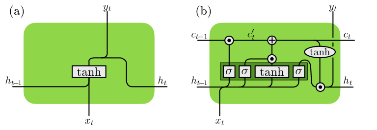
Fig. 21 Comparison of (a) a simple RNN and (b) a LSTM: The boxes denote neural networks with the respective activation function, while the circles denote element-wise operations. The dark green box indicates that the four individual neural networks can be implemented as one larger one.
Forget step
In this step, specific information of the cell state is forgotten.
Specifically, we update the cell state as
where \(\sigma\) is the sigmoid function (applied element-wise) and \(\odot\) denotes element-wise multiplication. Note that this step multiplies each element of the gate state with a number \(\in(0,1)\), in other words elements multiplied with a number close to \(0\) forget their previous memory.
Input and update step
In the next step, we decide what and how much to add to the cell state.
For this purpose, we first decide what to add to the state. We first
define what we would like to add to the cell,
which due to the hyperbolic tangent, \(-1 < g^\alpha_t < 1\) for each element. However, we do not necessarily update each element of the cell state, but rather we introduce another gate, which determines whether to actually write to the cell,
again with \(0<i^\alpha_t < 1\). Finally, we update the cell state
Output step
In the final step, we decide how much of the information stored in the
cell state should be written to the new hidden state,
The full structure of the LSTM with the four gates and the element-wise operations is schematically shown in Fig. 21(b). Note that we can concatenate the input \({\boldsymbol{x}}_t\) and hidden memory \({\boldsymbol{h}}_{t-1}\) into a vector of size \(n+m\) and write one large weight matrix \(W\) of size \(4m \times (m+n)\).
So far, we have only used the RNN in a supervised setting for classification purposes, where the input is a sequence and the output a single class at the end of the full sequence. A network that performs such a task is thus called a many-to-one RNN. We will see in the next section, that unlike the other network architectures encountered in this section, RNNs can straight-forwardly be used for unsupervised learning, usually as one-to-many RNNs.