
Adversarial Attacks
As we have seen, it is possible to modify the input \(\mathbf{x}\) so that the corresponding model approximates a chosen target output. This concept can also be applied to generate adverserial examples, i.e. images which have been intentionally modified to cause a model to misclassify it. In addition, we usually want the modification to be minimal or almost imperceptible to the human eye.
One common method for generating adversarial examples is known as the fast gradient sign method. Starting from an input \(\mathbf{x}^{0}\) which our model correctly classifies, we choose a target output \(\mathbf{y}^{*}\) which corresponds to a wrong classification, and follow the procedure described in the previous section with a slight modification. Instead of updating the input according to Eq. (49) we use the following update rule:
where \(L\) is given be Eq. (48). The \(\textrm{sign}(\dots) \in \lbrace -1, 1 \rbrace\) both serves to enhance the signal and also acts as constraint to limit the size of the modification. By choosing \(\eta = \frac{\epsilon}{T}\) and performing only \(T\) iterations, we can then guarantee that each component of the final input \(\mathbf{x}^{*}\) satisfies
which is important since we want our final image \(\mathbf{x}^{*}\) to be only minimally modified. We summarize this algorithm as follows:
Fast Gradient Sign Method
Input: A classification model \(\mathbf{f}\), a loss function \(L\), an initial image \(\mathbf{x}^{0}\), a target label \(\mathbf{y}_{\textrm{target}}\), perturbation size \(\epsilon\) and number of iterations \(T\)
Output: Adversarial example \(\mathbf{x}^{*}\) with \(|x^{*}_{i} - x^{0}_{i}| \leq \epsilon\)
\(\eta = \epsilon/T\)
for: i=1\dots T do
\(\quad\) \(\mathbf{x} = \mathbf{x} - \eta \ \textrm{sign}\left(\frac{\partial L}{\partial \mathbf{x}}\right)\)
end
This process of generating adversarial examples is called an adversarial attack, which we can classify under two broad categories: white box and black box attacks. In a white box attack, the attacker has full access to the network \(\mathbf{f}\) and is thus able to compute or estimate the gradients with respect to the input. On the other hand, in a black box attack, the adversarial examples are generated without using the target network \(\mathbf{f}\). In this case, a possible strategy for the attacker is to train his own model \(\mathbf{g}\), find an adversarial example for his model and use it against his target \(\mathbf{f}\) without actually having access to it. Although it might seem surprising, this strategy has been found to work albeit with a lower success rate as compared to white box methods. We shall illustrate these concepts in the example below.
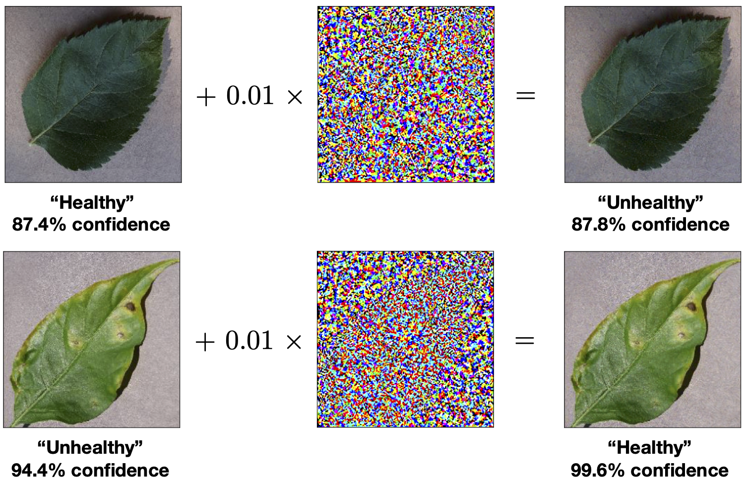
Fig. 31 Adversarial examples. Generated using the fast gradient sign method with \(T=1\) iteration and \(\epsilon = 0.01\). The target model is Google’s InceptionV3 deep convolutional network with a test accuracy of \(\sim 95\%\) on the binary (“Healthy” vs “Unhealthy”) plants dataset.
Example
We shall use the same plant leaves classification example as above. The target model \(\mathbf{f}\) which we want to ‘attack’ is a pretrained model using Google’s well known InceptionV3 deep convolutional neural network containing over \(20\) million parameters1. The model achieved a test accuracy of \(\sim 95\%\). Assuming we have access to the gradients of the model \(\mathbf{f}\), we can then consider a white box attack. Starting from an image in the dataset which the target model correctly classifies and applying the fast gradient sign method with \(\epsilon=0.01\) and \(T=1\), we obtain an adversarial image which differs from the original image by almost imperceptible amount of noise as depicted on the left of Fig. 31. Any human would still correctly identify the image but yet the network, which has around \(95\%\) accuracy has completely failed.
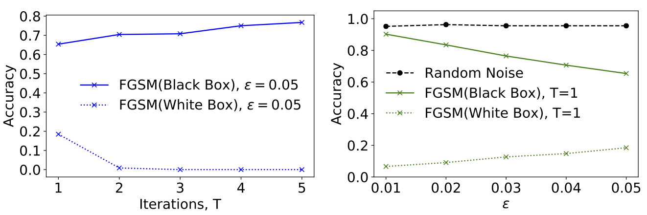
Fig. 32 Black Box Adversarial Attack.
If, however, the gradients and outputs of the target model \(\mathbf{f}\) are hidden, the above white box attack strategy becomes unfeasible. In this case, we can adopt the following ‘black box attack’ strategy. We train a secondary model \(\mathbf{g}\), and then applying the FGSM algorithm to \(\mathbf{g}\) to generate adversarial examples for \(\mathbf{g}\). Note that it is not necessary for \(\mathbf{g}\) to have the same network architecture as the target model \(\mathbf{f}\). In fact, it is possible that we do not even know the architecture of our target model.
Let us consider another pretrained network based on MobileNet containing about \(2\) million parameters. After retraining the top classification layer of this model to a test accuracy of \(\sim 95\%\), we apply the FGSM algorithm to generate some adversarial examples. If we now test these examples on our target model \(\mathbf{f}\), we notice a significant drop in the accuracy as shown on the graph on the right of Fig. 32. The fact that the drop in accuracy is greater for the black box generated adversarial images as compared to images with random noise (of the same scale) added to it, shows that adversarial images have some degree of transferability between models. As a side note, on the left of Fig. 32 we observe that black box attacks are more effective when only \(T=1\) iteration of the FGSM algorithm is used, contrary to the situation for the white box attack. This is because, with more iterations, the method has a tendency towards overfitting the secondary model, resulting in adversarial images which are less transferable.
These forms of attacks highlight a serious vulnerability of such data driven machine learning techniques. Defending against such attack is an active area of research but it is largely a cat and mouse game between the attacker and defender.
- 1
This is an example of transfer learning. The base model, InceptionV3, has been trained on a different classification dataset, ImageNet, with over \(1000\) classes. To apply this network to our binary classification problem, we simply replace the top layer with a simple duo-output dense softmax layer. We keep the weights of the base model fixed and only train the top layer.