
Computational neurons
The basic building block of a neural network is the neuron. Let us consider a single neuron which we assume to be connected to \(k\) neurons in the preceding layer, see Fig. 13 left side. The neuron corresponds to a function \(f:\mathbb{R}^k\to \mathbb{R}\) which is a composition of a linear function \(q:\mathbb{R}^k\to \mathbb{R}\) and a non-linear (so-called activation function) \(g:\mathbb{R}\to \mathbb{R}\). Specifically,
where \(z_1, z_2, \dots, z_k\) are the outputs of the neurons from the preceding layer to which the neuron is connected.
The linear function is parametrized as
Here, the real numbers \(w_1, w_2, \dots, w_k\) are called weights and can be thought of as the “strength” of each respective connection between neurons in the preceding layer and this neuron. The real parameter \(b\) is known as the bias and is simply a constant offset 2. The weights and biases are the variational parameters we will need to optimize when we train the network.
The activation function \(g\) is crucial for the neural network to be able to approximate any smooth function, since so far we merely performed a linear transformation. For this reason, \(g\) has to be nonlinear. In analogy to biological neurons, \(g\) represents the property of the neuron that it “spikes”, i.e., it produces a noticeable output only when the input potential grows beyond a certain threshold value. The most common choices for activation functions, shown in Fig. 13, include:
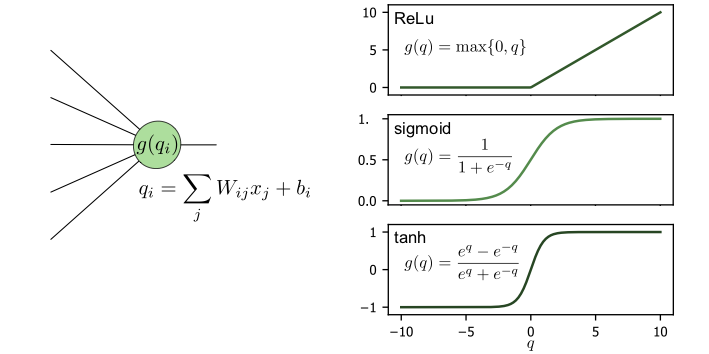
Fig. 13 Left: schematic of a single neuron and its functional form. Right: examples of the commonly used activation functions: ReLU, sigmoid function and hyperbolic tangent.
ReLU: ReLU stands for rectified linear unit and is zero for all numbers smaller than zero, while a linear function for all positive numbers.
Sigmoid: The sigmoid function, usually taken as the logistic function, is a smoothed version of the step function.
Hyperbolic tangent: The hyperbolic tangent function has a similar behaviour as sigmoid but has both positive and negative values.
Softmax: The softmax function is a common activation function for the last layer in a classification problem (see below).
The choice of activation function is part of the neural network architecture and is therefore not changed during training (in contrast to the variational parameters weights and bias, which are adjusted during training). Typically, the same activation function is used for all neurons in a layer, while the activation function may vary from layer to layer. Determining what a good activation function is for a given layer of a neural network is typically a heuristic rather than systematic task.
Note that the softmax provides a special case of an activation function as it explicitly depends on the output of the \(q\) functions in the other neurons of the same layer. Let us label by \(l=1,\ldots,n \) the \(n\) neurons in a given layer and by \(q_l\) the output of their respective linear transformation. Then, the softmax is defined as
for the output of neuron \(l\). A useful property of softmax is that \(\sum_l g_l(q_1,\ldots, q_n)=1,\) so that the layer output can be interpreted as a probability distribution. The softmax function is thus a continuous generalization of the argmax function introduced in the previous chapter.
A simple network structure
Now that we understand how a single neuron works, we can connect many of them together and create an artificial neural network. The general structure of a simple (feed-forward) neural network is shown in Fig. 14. The first and last layers are the input and output layers (blue and violet, respectively, in Fig. 14) and are called visible layers as they are directly accessed. All the other layers in between them are neither accessible for input nor providing any direct output, and thus are called hidden layers (green layer in Fig. 14.
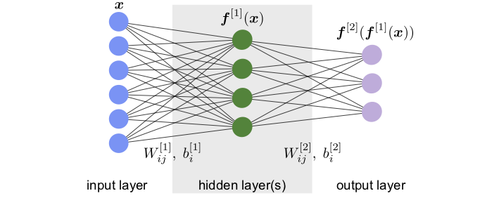
Fig. 14 Architecture and variational parameters.
Assuming we can feed the input to the network as a vector, we denote the input data with \({\boldsymbol{x}}\). The network then transforms this input into the output \({\boldsymbol{F}}({\boldsymbol{x}})\), which in general is also a vector. As a simple and concrete example, we write the complete functional form of a neural network with one hidden layer as shown in Fig. 14,
Here, \(W^{[n]}\) and \({\boldsymbol{b}}^{[n]}\) are the weight matrix and bias vectors of the \(n\)-th layer. Specifically, \(W^{[1]}\) is the \(k\times l\) weight matrix of the hidden layer with \(k\) and \(l\) the number of neurons in the input and hidden layer, respectively. \(W_{ij}^{[1]}\) is the \(j\)-the entry of the weight vector of the \(i\)-th neuron in the hidden layer, while \(b_i^{[1]}\) is the bias of this neuron. The \(W_{ij}^{[2]}\) and \({\boldsymbol{b}}_i^{[2]}\) are the respective quantities for the output layer. This network is called fully connected or dense, because each neuron in a given layer takes as input the output from all the neurons in the previous layer, in other words all weights are allowed to be non-zero.
Note that for the evaluation of such a network, we first calculate all the neurons’ values of the first hidden layer, which feed into the neurons of the second hidden layer and so on until we reach the output layer. This procedure, which is possible only for feed-forward neural networks, is obviously much more efficient than evaluating the nested function of each output neuron independently.
- 2
Note that this bias is unrelated to the bias we learned about in regression.