
Autoencoders
Autoencoders are neuron-based generative models, initially introduced for dimensionality reduction. The original purpose, thus, is similar to that of PCA or t-SNE that we already encountered in Sec. Structuring Data without Neural Networks, namely the reduction of the number of features that describe our input data. Unlike for PCA, where we have a clear recipe how to reduce the number of features, an autoencoder learns the best way of achieving the dimensionality reduction. An obvious question, however, is how to measure the quality of the compression, which is essential for the definition of a loss function and thus, training. In the case of t-SNE, we introduced two probability distributions based on the distance of samples in the original and feature space, respectively, and minimized their difference, for example using the Kullback-Leibler divergence.
The solution the autoencoder uses is to have a neural network do first, the dimensionality reduction, or encoding to the latent space, \(\mathbf{x}\mapsto \mathbf{e}(\mathbf{x})=\mathbf{z}\), and then, the decoding back to the original dimension, \(\mathbf{z} \mapsto \mathbf{d}(\mathbf{z})\), see Fig. 26. This architecture allows us to directly compare the original input \(\mathbf{x}\) with the reconstructed output \(\mathbf{d}(\mathbf{e}(\mathbf{x}))\), such that the autoencoder trains itself unsupervised by minimizing the difference. A good example of a loss function that achieves successful training and that we have encountered already several times is the cross entropy,
In other words, we compare point-wise the difference between the input to the encoder with the decoder’s output.
Intuitively, the latent space with its lower dimension presents a bottleneck for the information propagation from input to output. The goal of training is to find and keep the most relevant information for the reconstruction to be optimal. The latent space then corresponds to the reduced space in PCA and t-SNE. Note that much like in t-SNE but unlike in PCA, the new features are in general not independent.
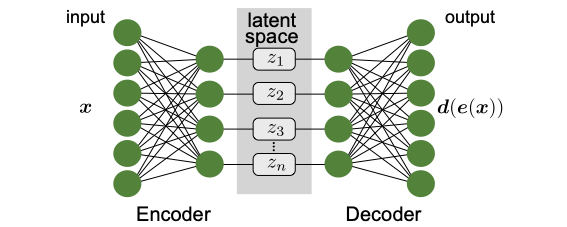
Fig. 26 General autoencoder architecture. A neural network is used to contract a compressed representation of the input in the latent space. A second neural network is used to reconstruct the original input.
Variational Autoencoders
A major problem of the approach introduced in the previous section is its tendency to overfitting. As an extreme example, a sufficiently complicated encoder-decoder pair could learn to map all data in the training set onto a single variable and back to the data. Such a network would indeed accomplish completely lossless compression and decompression. However, the network would not have extracted any useful information from the dataset and thus, would completely fail to compress and decompress previously unseen data. Moreover, as in the case of the dimensionality-reduction schemes discussed in Sec. Structuring Data without Neural Networks, we would like to analyze the latent space images and extract new information about the data. Finally, we might also want to use the decoder part of the autoencoder as a generator for new data. For these reasons, it is essential that we combat overfitting as we have done in the previous chapters by regularization.
The question then becomes how one can effectively regularize the autoencoder. First, we need to analyze what properties we would like the latent space to fulfil. We can identify two main properties:
If two input data points are close (according to some measure), their images in the latent space should also be close. We call this property continuity.
Any point in the latent space should be mapped through the decoder onto a meaningful data point, a property we call completeness.
While there are principle ways to achieve regularization along similar paths as discussed in the previous section on supervised learning, we will discuss here a solution that is particularly useful as a generative model: the variational autoencoder (VAE).
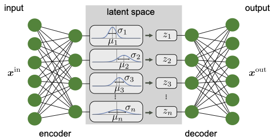
Fig. 27 Architecture of variational autoencoder. Instead of outputting a point \(z\) in the latent space, the encoder provides a distribution \(N(\boldsymbol \mu, \boldsymbol \sigma)\), parametrized by the means \(\boldsymbol \mu\) and the standard deviations \(\boldsymbol \sigma\). The input \(\mathbf{z}\) for the decoder is then drawn from \(N(\boldsymbol \mu, \boldsymbol \sigma)\).
The idea behind VAEs is for the encoder to output not just an exact point \(\mathbf{z}\) in the latent space, but a (factorized) Normal distribution of points, \(\mathcal{N}(\boldsymbol \mu, \boldsymbol \sigma)\). In particular, the output of the encoder comprises two vectors, the first representing the means, \(\boldsymbol \mu\), and the second the standard deviations, \(\boldsymbol \sigma\). The input for the decoder is then sampled from this distribution, \(\mathbf{z} \sim \mathcal{N}(\boldsymbol \mu, \boldsymbol \sigma)\), and the original input is reconstructed and compared to the original input for training. In addition to the standard loss function comparing input and output of the VAE, we further add a regularization term to the loss function such that the distributions from the encoder are close to a standard normal distribution \(\mathcal{N}(\boldsymbol 0, \boldsymbol 1)\). Using the Kullback-Leibler divergence, Eq. (6), to measure the deviation from the standard normal distribution, the full loss function then reads
In this expression, the first term quantifies the reconstruction loss with \(\mathbf{x}_i^{\rm in}\) the input to and \(\mathbf{x}_i^{\rm out}\) the reconstructed data from the VAE. The second term is the regularization on the latent space for each input data point, which for two (diagonal) Normal distributions can be simplified, see second line of Eq. (46). This procedure regularizes the training through the introduction of noise, similar to the dropout layer in Section Computational neurons. However, the regularization here not only generically increases generalization, but also enforces the desired structure in the latent space.
The structure of a VAE is shown in Fig. 27. By enforcing the mean and variance structure of the encoder output, the latent space fulfills the requirements outlined above. This type of structure can then serve as a generative model for many different data types: anything from human faces to complicated molecular structures. Hence, the variational autoencoder goes beyond extracting information from a dataset, but can be used for the scientific discovery. Note, finally, that the general structure of the variational autoencoder can be applied beyond the simple example above. As an example, a different distribution function can be enforced in the latent space other than the standard Normal distribution, or a different neural network can be used as encoder and decoder, such as a RNN.