
Advanced Layers
In the previous sections, we have illustrated an artificial neural network that is constructed analogous to neuronal networks in the brain. A model is only given a rough structure a priori, within which they have a huge number of parameters to adjust by learning from the training set. While we already understand that this is an extraordinarily powerful process, this method of learning comes with its own set of challenges. The most prominent of them is the generalization of the rules learned from training data to unseen data.
We have already encountered in the previous chapter how the naive optimization of a linear model reduces the generalization. However, we have also seen how the generalization error can be improved using regularization. Training neural network comes with the same issue and the same solution: we are always showing the algorithm we built the training that is limited in one way or another and we need to make sure that the neural network does not learn particularities of that given training set, but actually extracts a general knowledge.
The step zero to avoid over-fitting is to create sufficiently representative and diverse training set. Once this is taken care of, we can take several steps for the regularization of the network. The simplest, but at the same time most powerful option is introducing dropout layers. This regularization is very similar to dropping features that we discussed for linear regression. However, the dropout layer ignores a randomly selected subset of neuron outputs in the network only during training. Which neurons are dropped is chosen at random for each training step. This regularization procedure is illustrated in Fig. 15. By randomly discarding a certain fraction of neurons we ensure that the network does not get fixed at small particular features of the training set and is better equipped to recognize the more general features. Another way of looking at it is that this procedure corresponds to training a large number of neural networks with different neuron connections in parallel. The fraction of neurons that are ignored in a dropout layer is a hyperparameter that is fixed a priori. Maybe it is counter-intuitive but the best performance is often achieved when this number is sizable, between 20% and 50%. It shows the remarkable resilience of the network against fluctuations.
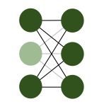
Fig. 15 Dropout layer.
As for the linear models, regularization can also be achieved by adding regularization terms \(R\) to the \(L\), \(L \rightarrow L + R\). Again, the two most common regularization terms are \(L1\)- or Lasso-regularisation, where
and the sum runs over all weights \(W_j\) of the network, as well as the \(L2\)-regularization, or ridge regression, which we already discussed for linear regression with
where the sum runs again over all weights \(W_j\) of the network. As for the linear models, \(L2\) regularization shrinks all parameters symmetrically, whereas \(L1\)-regularization usually causes a subset of parameters to vanish. For this reason, the method is also called weight decay. Either way, both \(L1\) and \(L2\) regularizations restrict the expressiveness of the neural network, thus encouraging it to learn generalizable features rather than overfitting specific features of the data set.
The weights are commonly initialized with small values and increase during training. This naturally limits the capacity of the network, because for very small weights it effectively acts as a linear model (when one approximates the activation function by a linear function). Only once the weights become bigger, the network explores its nonlinearity.
Another regularization technique consists in artificially enlarging the data set. Data is often costly, but we have extra knowledge about what further data might look like and feed this information in the machine learning workflow. For instance, going back to the MNIST example, we may shift or tilt the existing images or apply small transformations to them. By doing that, researchers were able to improve MNIST performance by almost 1 percent 3. In particular if we know symmetries of the problem from which the data originates (such as time translation invariance, invariance under spatial translations or rotations), effective generation of augmented datasets is possible. Another option is the addition of various forms of noise to data in order to prevent overfitting to the existing noise or in general resilience of the neural network to noise. Finally, for classification problems in particular, data may not be distributed between categories equally. To avoid a bias, it is the desirable to enhance the data in the underrepresented categories.
Convolutional neural networks
The fully-connected simple single-layer architecture for a neural network is in principle universally applicable. However, this architecture is often inefficient and hard to train. In this section, we introduce more advanced neural-network layers and examples of the types of problems for which they are suitable.
Convolutional layers
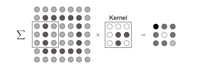
Fig. 16 Convolutional layer in 2D: Here with filter size \(k=3\) and stride \(s=2\). The filter is first applied to the \(3\times 3\) sub-image in the top left of the input, which yields the first pixel in the feature map. The filter then moves \(s\) neurons to the right, which yields the next pixel and so on. After moving all the way to the right, the filter moves \(s\) pixels down and starts from the left again until reaching the bottom right.
The achieved accuracy in the MNIST example above was not as high as one may have hoped, being much worse than the performance of a human. A main reason was that, using a dense network structure, we discarded all local information contained in the pictures. In other words, connecting every input neuron with every neuron in the next layer, the information whether two neurons are close to each other is lost. This information is, however, not only crucial for pictures, but quite often for input data with an underlying geometric structure or natural notion of ‘distance’ in its correlations. To use this local information, so-called convolutional layers were introduced. The neural networks that contain such layers are called convolutional neural networks (CNNs).
The key idea behind convolutional layers is to identify certain (local) patterns in the data. In the example of the MNIST images, such patterns could be straight and curved lines, or corners. A pattern is then encoded in a kernel or filter in the form of weights, which are again part of the training. The convolutional layer than compares these patterns with a local patch of the input data. Mathematically, identifying the features in the data corresponds to a convolution \((f * x)(t)=\sum_{\tau}f(\tau)x(t-\tau)\) of the kernel \(f\) with the original data \(x\).
For two-dimensional data, such as shown in the example in Fig. 16, we write the discrete convolution explicitly as
where \(f_{n,m}\) are the weights of the kernel, which has linear size \(k\), and \(b_0\) is a bias. Finally, \(s\) is called stride and refers to the number of pixels the filter moves per application. The output, \(q\), is called feature map. Note that the dimension of the feature map is \(n_q\times n_q\) with \(n_q = \lfloor (n_{in} - k)/s + 1 \rfloor \) when the input image is of dimensions \(n_{in} \times n_{in}\): application of a convolutional layer thus reduces the image size, an effect not always intended. To avoid this reduction, the original data can be padded, for example by adding zeros around the border of the data to ensure the feature map has the same dimension as the input data.
For typical convolutional networks, one applies a number of filters for each layer in parallel, where each filter is trained to recognize different features. For instance, one filter could start to be sensitive to contours in an image, while another filter recognizes the brightness of a region. Further, while filters in the first layers may be sensitive to local patterns, the ones in the later layers recognize larger structures. This distribution of functionalities between filters happens automatically, it is not preconceived when building the neural network.
Pooling
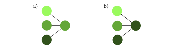
Fig. 17 Pooling layer: (a) an average pooling and (b) a max pooling layer (both \(n=3\)).
Another very useful layer, in particular in combination with convolutional layers, is the pooling layer. Each neuron in the pooling layer takes input from \(n\) (neighboring) neurons in the previous layer—in the case of a convolutional network for each feature map individually—and only retains the most significant information. Thus, the pooling layer helps to reduce the spatial dimension of the data. What is considered significant depends on the particular circumstances: Picking the neuron with the maximum input among the \(n\), called max pooling, detects whether a given feature is present in the window. Furthermore, max pooling is useful to avoid dead neurons, in other words neurons that are stuck with a value near 0 irrespective of the input and such a small gradient for its weights and biases that this is unlikely to change with further training. This is a scenario that can often happen especially when using the ReLU activation function. Average pooling, in other words taking the average value of the \(n\) inputs is a straight forward compression. Note that unlike other layers, the pooling layer has just a small set of \(n\) connections with no adjustable weights. The functionality of the pooling layer is shown in Fig. 17 (a) and (b).
An extreme case of pooling is global pooling, where the full input is converted to a single output. Using a max pooling, this would then immediately tell us, whether a given feature is present in the data.
Example: DNA sequencing
With lowering costs and expanding applications, DNA sequencing has become a widespread tool in biological research. Especially the introduction of high-throughput sequencing methods and the related increase of data has required the introduction of data science methods into biology. Sequenced data is extremely complex and thus a great playground for machine learning applications. Here, we consider a simple classification as an example. The primary structure of DNA consists of a linear sequence of basic building blocks called nucleotides. The key component of nucleotides are nitrogen bases: Adenine (A), Guanine (G), Cytosine (C), and Thymine (T). The order of the bases in the linear chains defines the DNA sequence. Which sequences are meaningful is determined by a set of complex specific rules. In other words, there are series of letters A, G, C, and T that correspond to DNA and while many other sequences do not resemble DNA. Trying to distinguish between strings of nitrogen bases that correspond to human DNA and those that don not is a simple example of a classification task that is at the same time not so easy for an untrained human eye.
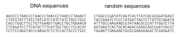
Fig. 18 Comparison of DNA and random sequences.
In Fig. 18, we show a comparison of five strings of human DNA and five strings of 36 randomly generated letters A, G, C, and T. Without deeper knowledge it is hard to distinguish the two classes and even harder to find the set of empirical rules that quantify their distinction. We can let a neural network have a go and see if it performs any better than us studying these sequences by visual analysis.
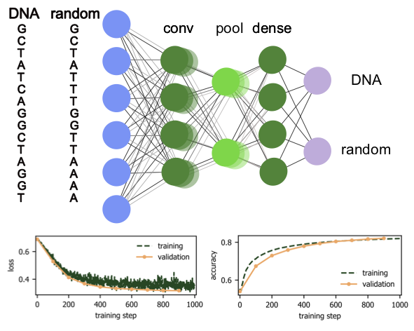
Fig. 19 Neural network classification of DNA sequences: The upper panel shows the architecture and he two lower panels show loss function and accuracy on the training (evaluation) data in green (orange) as a function of the training step respectively.
We have all ingredients to build a binary classifier that will be able to distinguish between DNA and non-DNA sequences. First, we download a freely available database of the human genome from https://genome.ucsc.edu4. Here, we downloaded a database of encoding genomes that contains \(100 000\) sequences of human DNA (each is 36 letters long). Additionally, we generate \(100 000\) random sequences of letters A, G, C, T. The learning task we are facing now is very similar to the MNIST classification, though in the present case, we only have two classes. Note, however, that we generated random sequences of bases and labeled them as random, even though we might have accidentally created sequences that do correspond to human DNA. This limits the quality of our data set and thus naturally also the final performance of the network.
The model we choose here has a standard architecture and can serve as a guiding example for supervised learning with neural networks that will be useful in many other scenarios. In particular, we implement the following architecture:
DNA Classification
Import the data from http://genome.uscs.edu
Define the model:
Input layer: The input layer has dimension \(36\times 4\) (\(36\) entries per DNA sequence, \(4\) to encode each of 4 different bases A, G, C, T)
Example: [[1,0,0,0], [0,0,1,0], [0,0,1,0], [0,0,0,1]] = ACCTConvolutional layer: Kernel size \(k= 4\), stride \(s= 1\) and number of filters \(N=64\).
Pooling layer: max pooling over \(n=2\) neurons, which reduces the output of the previous layer by a factor of 2.
Dense layer: 256 neurons with a ReLU activation function.
Output layer: 2 neurons (DNA and non-DNA output) with softmax activation function.
Loss function: Cross-entropy between DNA and non-DNA.
A schematic of the network structure as well as the evolution of the loss and the accuracy measured over the training and validation sets with the number of training steps are shown in Fig. 19. Comparing the accuracies of the training and validation sets is a standard way to avoid overfitting: On the examples from the training set we can simply check the accuracy during training. When training and validation accuracy reach the same number, this indicates that we are not overfitting on the training set since the validation set is never used to adjust the weights and biases. A decreasing validation accuracy despite an increasing training accuracy, on the other hand, is a clear sign of overfitting.
We see that this simple convolutional network is able to achieve around 80% accuracy. By downloading a larger training set, ensuring that only truly random sequences are labeled as such, and by optimizing the hyper-parameters of the network, it is likely that an even higher accuracy can be achieved. We also encourage you to test other architectures: one can try to add more layers (both convolutional and dense), adjust the size of the convolution kernel or stride, add dropout layers, and finally, test whether it is possible to reach higher accuracies without over-fitting on the training set.
Example: advanced MNIST
We can now revisit the MNIST example and approach the classification with the more advanced neural network structures of the previous section. In particular, we use the following architecture
Advanced MNIST
Input layer: \(28^2 = 784\) neurons.
Convolutional layer 1: Kernel size \(k= 5\), stride \(s= 1\) and number of filters \(N=32\) with a ReLU activation function.
Pooling layer: max pooling over \(n=2\times 2\) neurons.
Convolutional layer 2: Kernel size \(k= 5\), stride \(s= 1\) and number of filters \(N=64\) with a ReLU activation function.
Pooling layer: max pooling over \(n=2\times 2\) neurons.
Dropout: dropout layer for regularization with a 50% dropout probability.
Dense layer: 1000 neurons with a ReLU activation function.
Output layer: 10 neurons with softmax activation function.
For the loss function, we again use cross-entropy between the output and the labels. Notice here the repeated structure of convolutional layers and pooling layers. This is a very common structure for deep convolutional networks. With this model, we achieve an accuracy on the MNIST test set of 98.8%, a massive improvement over the simple dense network.