
Finite Markov Decision Process
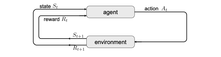
Fig. 34 Markov decision process. Schematic of the agent-environment interaction.
After this introductory example, we introduce the idealized form of reinforcement learning with a Markov decision process (MDP). At each time step \(t\), the agent starts from a state \(S_t\in \mathcal{S}\), performs an action \(A_t\in\mathcal{A}\), which, through interaction with the environment, leads to a reward \(R_{t+1}\in \mathcal{R}\) and moves the agent to a new state \(S_{t+1}\). This agent-environment interaction is schematically shown in Fig. 34. Note that we assume the space of all actions, states, and rewards to be finite, such that we talk about a finite MDP.
For our toy example, the sensor we have only shows whether the water level is high (h) or low (l), so that the state space of our agent is \(\mathcal{S} = \{ {\rm h}, {\rm l} \}\). In both cases, our agent can choose to turn the growth lamps on or off, or in the case of low water, he can choose to send us a message so we can go and water the plants. The available actions are thus \(\mathcal{A} = \{{\rm on}, {\rm off}, {\rm text}\}\). When the growth lamps are on, the plants grow faster, which leads to a bigger reward, \(r_{\rm on} > r_{\rm off}>0\). Furthermore, there is a penalty for texting us, but an even bigger penalty for letting the plants die, \(0 > r_{\rm text} > r_{\rm fail}\).
A model of the environment provides the probability of ending in state \(s'\) with reward \(r\), starting from a state \(s\) and choosing the action \(a\), \(p(s', r | s, a)\). In this case, the dynamics of the Markov decision process is completely characterized. Note that the process is a Markov process, since the next state and reward only depend on the current state and chosen action.
In our toy example, being in state ‘high’ and having the growth lamp on will provide a reward of \(r_{\rm on}\) and keep the agent in ‘high’ with probability \(p({\rm h}, r_{\rm on} | \rm {h}, {\rm on}) = \alpha\), while with \(1-\alpha\) the agent will end up with a low water level. However, if the agent turns the lamps off, the reward is \(r_{\rm off}\) and the probability of staying in state ‘high’ is \(\alpha' > \alpha\). For the case of a low water level, the probability of staying in low despite the lamps on is \(p({\rm l}, r_{\rm on} | \rm {l}, {\rm on}) = \beta\), which means that with probability \(1 - \beta\), our plants run out of water. In this case, we will need to get new plants and we will water them , of course, such that \(p({\rm h}, r_{\rm fail} | \rm {l}, {\rm on}) = 1-\beta\). As with high water levels, turning the lamps off reduces our rewards, but increases our chance of not losing the plants, \(\beta' > \beta\). Finally, if the agent should choose to send us a text, we will refill the water, such that \(p({\rm h}, r_{\rm text} | {\rm l}, {\rm text}) = 1\). The whole Markov process is summarized in the transition graph in Fig. 35.
From the probability for the next reward and state, we can also calculate the expected reward starting from state \(s\) and choosing action \(a\), namely
Obviously, the value of an action now depends on the state the agent is in, such that we write \(q_* (s, a)\). Alternatively, we can also assign to each state a value \(v_*(s)\), which quantizes the optimal reward from this state.
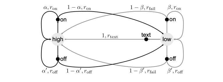
Fig. 35 Transition graph of the MDP for the plant-watering agent. The states ‘high’ and ‘low’ are denoted with large circles, the actions with small black circles, and the arrows correspond to the probabilities and rewards.
Finally, we can define what we want to accomplish by learning: knowing our current state \(s\), we want to know what action to choose such that our future total reward is maximized. Importantly, we want to accomplish this without any prior knowledge of how to optimize rewards directly. This poses yet another question: what is the total reward? We usually distinguish tasks with a well-defined end point \(t=T\), so-called episodic tasks, from continuous tasks that go on for ever. The total reward for the former is simply the total return
As such a sum is not guaranteed to converge for a continuous task, the total reward is the discounted return
with \(0 \leq \gamma < 1\) the discount rate. Equation (50) is more general and can be used for an episodic task by setting \(\gamma = 1\) and \(R_t = 0\) for \(t>T\). Note that for rewards which are bound, this sum is guaranteed to converge to a finite value.